Kalman filters: Information can only reduce your uncertainty

• 14 Mar, 2024
• by Igor Mijić

Some 8 or 9-ish years ago, as a budding signal processing practitioner, fresh-faced and naively enamored with this “new big thing” called deep learning, I’d listen to my PhD candidate research colleagues who were coming from robotics and automatics backgrounds, talking about how trivial it would be to apply Kalman filters to this problem or another.

At the time, I thought it kind of fell under the old Maslow quote: “I suppose it is tempting, if the only tool you have is a hammer, to treat everything as if it were a nail.”

They had just spent several semesters learning it in courses, applying it to laboratory problems, using it in projects, etc. So, I shrugged it off initially.

I, myself, managed to slide through school without using it and without attending courses that would cover it. But hey, it’s a filter, and filters are what signal processing is about. So after some time, I decided to try and acquaint myself with it.

I had spent some time rummaging through “dry” math textbooks and online video course materials before I stumbled onto a clip of a professor that summed it up as the section title states. “Information can only reduce your uncertainty!“.

Well, my interest instantly skyrocketed.

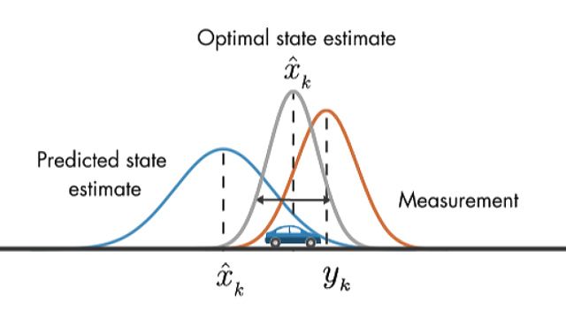
That statement is, in fact, very vague and suggests applicability to a lot of problems, similar to how my colleagues talked about it. The professor was actually talking about how in Kalman filters, the measurement reduces your uncertainty about the prediction of the filter.

Another key takeaway point was also that it works both ways, and the prediction reduces the uncertainty about the measurement.

Now, “measurement” and “prediction” (sometimes “estimate”), if you’re not yet familiar with Kalman filters or their applications, are all vague. So, throughout this article, we’ll tell you what they are and how they fit within the common Kalman Filter algorithms. Plus, we’ll show you how they are applied to face tracking within visage|SDK.

What are Kalman filters: A basic example

Imagine a situation like this.

You are using GPS to track a moving vehicle. But the GPS is giving you noisy information about the vehicle position, for every “measurement” or step that you query.

You may also have some idea about the nature of the vehicle’s movement, such as the movement pattern, environmental factors, speed, acceleration, etc. – a sort of “model.” However, models are also inherently not precise enough. The estimates they produce have errors with distributions connected to the level of approximation of the modeled phenomenon, in this case, the car’s movement.

In that case, you can use a Kalman filter to combine the GPS measurements and the model to get a better estimate of the vehicle’s position. The GPS measurement reduces your uncertainty about the prediction of the position coming from your model. But at the same time, the prediction from your model reduces the uncertainty about the GPS measurement.

The more measurements you have, the more accurate your estimate will be. But there’ll always be some uncertainty due to the noise in the GPS and the unsatisfactory nature of the model.

^{Source: MathWorks}

Various flavors of Kalman filters

When talking about applications of Kalman filters in robotics, control, computer vision, etc., we usually need to be a bit more specific about which actual filter we are using.

This isn’t just because the mathematicians out there are forcing specificity, but due to various generalizations and implementations of the general estimation and prediction steps in the algorithm workflow that each fit well to their respective applications.

In short, there is a whole host of specific filters that all follow a workflow similar to the example above but go about it slightly differently.

A formal diagram of the workflow can be described as in Figure 1:

1. Initialize system state to some “guestimate” value.
2. Take measurements of your input variables.
3. Estimate the current state of the system by using the previous state (if first iteration, then the “guestimate”) and the measurement.
4. Predict the state for the next iteration.

Repeat steps 1-3.

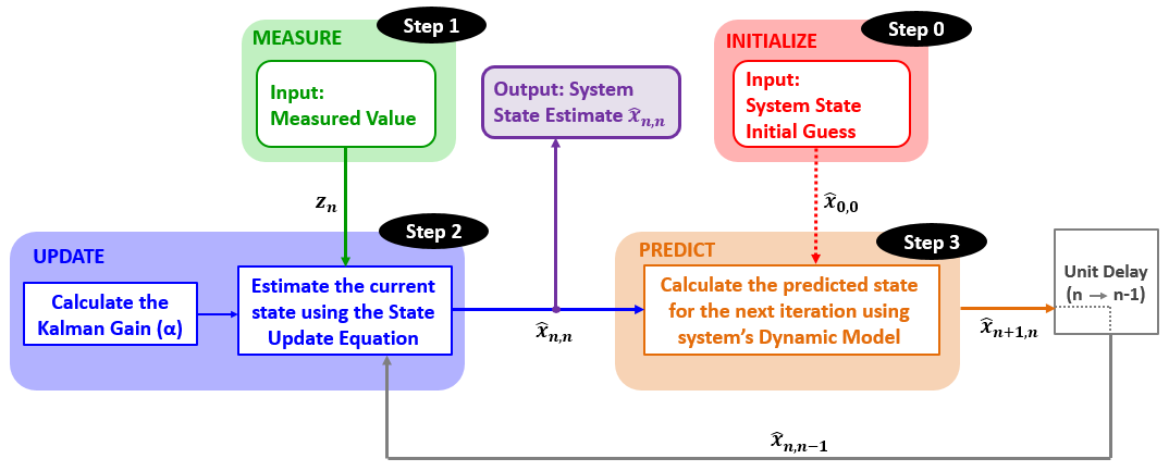
^{Figure 1: A measure-predict type workflow commonly used in Kalman-type algorithms (image source: Online Kalman Filter Tutorial)}

The most commonly used “flavors” of Kalman filters are:

• The Linear Kalman Filter (KF) – a recursive Bayesian filter that estimates the state of a linear system with Gaussian noise. It consists of two steps: prediction and update. In the prediction step, the filter uses a state transition model to predict the next state and its uncertainty. In the update step, the filter uses a measurement model to incorporate new observations and correct the predicted state and its uncertainty.
• The Extended Kalman Filter (EKF) – an extension of the Kalman filter for nonlinear systems. It uses the same prediction and update steps, but it linearizes the nonlinear state transition and measurement. This is achieved at the cost of optimality, which the KF has for the linear case. While suboptimal in its solution, it does enable the usage on more real-world applications for which the state transition behavior or the measurement behavior is non-linear (which is common in robotics, navigation, and computer vision)
• The Extended Information Filter (EIF) – another extension of the Kalman filter for nonlinear systems. It is similar to the extended Kalman filter, but it works in the dual space of information, which is the inverse of the covariance matrix. The information matrix represents the precision of the state estimate, and the information vector represents the weighted sum of the measurements.

Now, you math-savvy readers might say: “Well, Igor, this is all very apparent when you look at the different state equations for the different Kalman variants.”

And it is, which we will comment on in the next section. So if you are one of those, and like reviewing equations or want to learn more about the mathematical background of the Kalman variants, then stick with me. But if you are one of the “practical” technology users who like to look at modeling techniques as black-box tools, you might want to focus on the definitions mentioned above and skip right to the next sections for an overview of how we use EIF in visage|SDK.

The math behind Kalman filters

In short, if a problem can be defined as the following, the Kalman filter can be used:

Each component is the following:

• z_k is observation (or measurement) at the time k,
• x_k is the process state,
• H_k is the observation model or matrix that connects the internal state with observation,
• v_k is observation noise (measurements in the real world are never perfect, and they always have some noise component).

Now, if we assume model linearity, this holds and fully describes the Kalman Filter. But if our observation model is not linear, we have to extend it to:

where h() is a non-linear function. Now we are finally working with an Extended Kalman Filter. And finally, if we implement it with matrix inverses, we are talking about an Extended Information Filter.

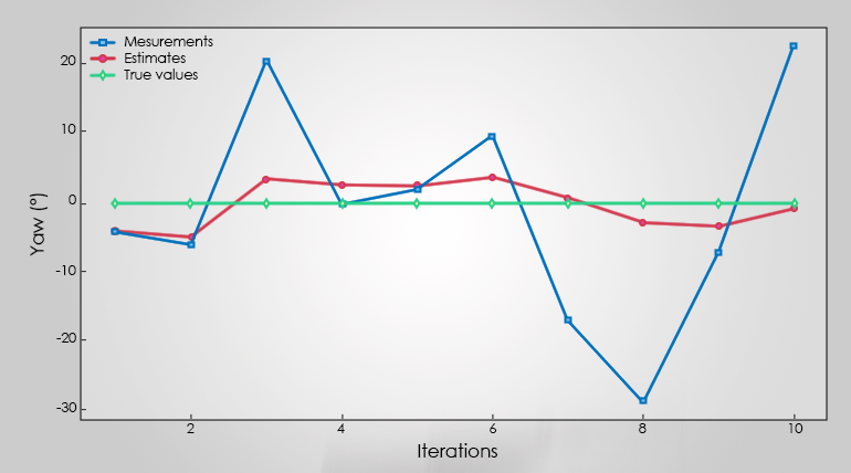
Whichever filter we have, it will produce something similar to what we see in Figure 2. For a set of measurements, it will converge iteratively, to a solution better than the initially estimated one.

Face Fitting example from visage|SDK

Now that you know a bit more about Kalman filters, how they work, what types there are, etc., let’s talk about how we apply them in visage|SDK.

In essence, the VisageModelFitter class of our SDK works in concert with other key components of the SDK. After the face detection and face alignment steps are performed, a set of feature points, or Facial Feature Landmarks (FPs), is produced for each face detected.

The fitting algorithm uses those FPs to estimate 4 sets of face model parameters (sometimes called deformations). These are applied to a face model to make it resemble the original face as closely as possible while also being positioned in space as precisely as possible.

The 4 sets of parameters are as follows:

• Face shape: We use a set of deformations of a 3D mesh called Shape Units (SUs).
• Face expression: Another set of deformations in the 3D mesh called Action Units (AUs) is used for this.
• Face rotation in the 3 axis (rotation in X is pitch, in Y is yaw, and in Z is roll).
• Face translation in the 3 axis.

If we reference the maths from the previous section, we get that in our use-case

• z_k are the 2D Facial Feature Points,
• x_k would be the rotation, translation, shape, and action unit’s coefficient of the 3D model we’re fitting on 2D points,
• H_k is a matrix which connects these two, and
• v_k would be the noise of the 2D landmarks.

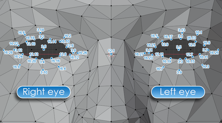
If we observe Figure 3, we see yellow dots (FPs), three axes of rotation (x_k), and finally, the mesh model.

Now, while the initial guess of nonlinearity was initially apparent (doh, no way something that complex is linear), the reason for using the Extended Information filter might not have been until now. It is, in fact, the number of observations (FP coordinates) that is much larger than the number of states (rotation, translation, SUs, and AUs), which makes it easier to deal with an inversed matrix. 🙂

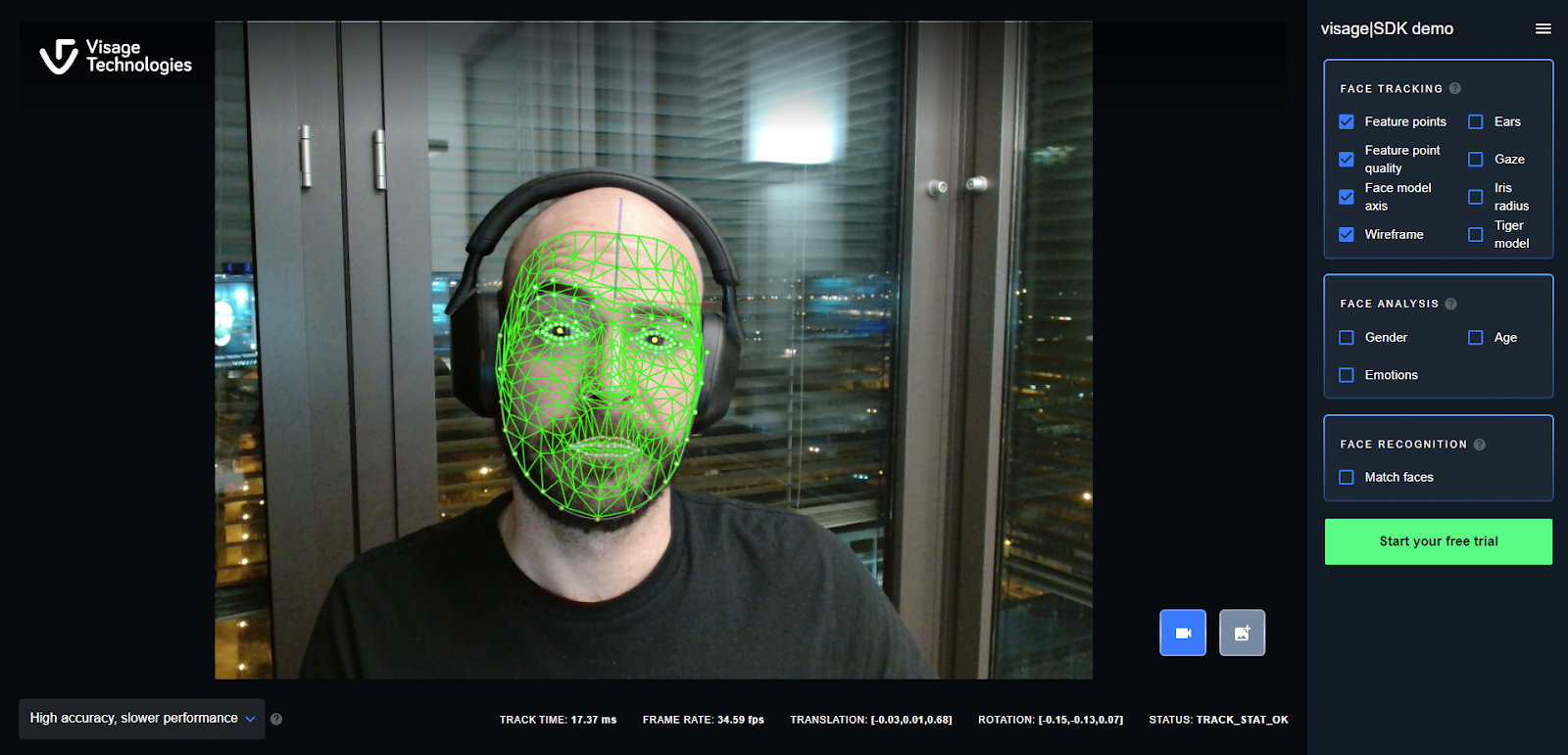
^{Figure 3}

Now we are finally at a point when it becomes more apparent how the Kalman Filter fits into the visage|SDK.

Within the formal definition of the problem, we can see that the FPs fit neatly into the “measurement” category of input mentioned in the previous sections. And the 4 sets of parameters provide the descriptive variables for our system state, which get predicted after every iteration.

The only thing that might still be unclear is what we use to model the system. And what the link between the measurements and the state is.

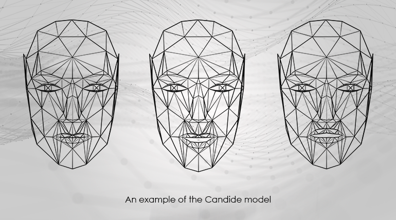
That is where the 3D face mesh model “enters” the game. The Candide model holds information about the initial, neutral state sizes, shapes, and positions of the triangles of the face mesh in 3D, while also holding information on how they get deformed. That is our “model” from our car/GPS example from the initial section of the article.

Kalman in practice: First frame fitting

Now let’s talk about an actual engineering problem one has to solve when using EIF for face tracking. It’s heavily related to the article’s title and the initial guestimate mentioned in the Various flavors of Kalman filters section, as the 0th step of the workflow. First frame fitting, or the initial “guesstimate” of the state of the system.

When we first detect a face and get the FPs from the alignment network, that first measurement does not have a matching prediction. And we need one to kickstart the process as described in the starting sections.

Also, we need to keep in mind that the quality of this 0th step estimate will not only affect the next step prediction but also the speed and the ability of convergence of the fitting algorithm.

So how does one go about it?

Well, the simplest option would be to assume all starting frames as frontal. So, we can use the face proportions as translation estimates and the rotation estimates as 0 degrees.

It turns out it’s not that good of an estimate at all. Except when the fitting starts directly from the frontal position. However, we can’t very well ask our clients to always start the fitting with a frontal face. 🙂

That’s why we must use information about more than a couple pairs of FPs, their relation in 2D space, etc.

The differences are so drastic that simply by improving the original assumption of a frontal face with one that takes into account one more FP, we can see 50% first frame fitting improvements and quicker convergence, both showing the importance of how measurement and prediction reduce the uncertainty of one another.

Dive deeper

If you’ve made it this far, I’m gonna assume you found some of this Kalman Face Tracking mumbo jumbo interesting. Or you have an idea of how you would use it within your product.

In that case, don’t hesitate to contact me directly with any questions, feedback, reflections, or just to say hello. You can also try our technology live or get in touch with our sales team for a free trial.