Tensors in computer vision

• 09 Aug, 2021
• by Maja Zalac

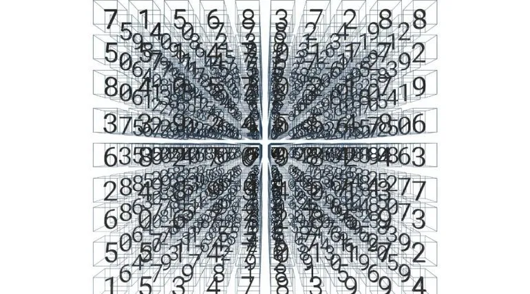
When it comes to the concept of using tensors in computer vision, it is crucial to understand what tensors generally are, how they are shaped and used.

What are tensors?

Tensors are mathematical objects. They are d-dimensional arrays of numbers, objects in which each element is defined by d-indices, for example, vectors (1-d tensor) and matrices (2-d tensor). The terminology used for marking the number of tensor’s dimensions is an order of the tensor (5d-tensor is a tensor of order 5), and each of these dimensions is referred to as a mode (a tensor of order 5 has 5 modes).

Graphically, it is easiest to represent tensors by using some kind of geometric shape (for example, a circle) while modes are represented by lines (often called legs). In that case, a vector could be easily graphically represented as a combination of one circle and one line because it has one dimension.

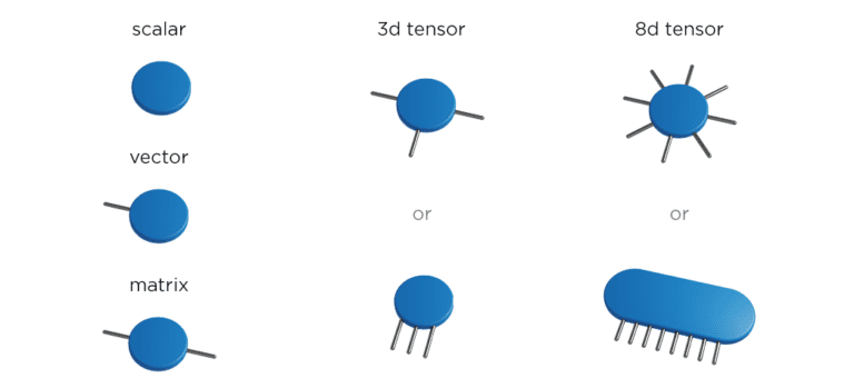
This way of representing tensors also allows the display of various operations involving tensors, for example, multiplications. In the case of matrix-vector multiplication, the resulting object of the matrix time vector is a vector. In that simple example, two mutual lines are contracted in one, two tensors get multiplied, and the result is one tensor with one line – a vector.

Why use tensors?

The power of tensors lies in the fact that they naturally represent data. It is possible to find different examples of where data is described using tensors. One example is images. Each digital image is represented as three matrices of pixels – red, green, and blue. If you look at it as one object, it is a tensor of order 3. It is possible to expand this kind of tensor to d-dimensions by adding different dimensions, such as multiple persons, expressions, different lightning, etc. Below is a 5d tensor that includes x position, y position, R/G/B, person, and expression.

The main problem with tensors is their size. The number of entries increases exponentially with d – the number of dimensions. Even for n=2, storing a tensor of order 50 would require 9 petabytes. This situation is called “the curse of dimensionality” because it prevents explicit storage of entries except for very small values of d.

The solution to this problem are tensor decompositions and tensor contractions. These are two main tools that make tensor algorithms efficient. Tensor contractions are different multiplications that need to be performed when dealing with tensors which can be done efficiently by correctly connecting different objects. Tensor decompositions allow us to store these huge objects – instead of storing one large object, you can store several smaller ones.

Tensor decompositions

Tensor decompositions are very similar to matrix decompositions. However, the class of low-rank tensors is much richer than the class of low-rank matrices. So, it is possible to perform different decompositions depending on what type of properties a tensor has. Depending on a problem that needs to be resolved, it is necessary to use different decompositions. The most known decompositions and the reasons why they are used are listed below.

• Tucker decomposition – for compression of tensors
• Canonical Polyadic (CP) decomposition – for interpretation of data-related tensors
• Hierarchical Tucker decomposition – decomposes a tensor into a tree structure of objects
• Tensor Train (TT) decomposition – for tensors of very high order

In Tucker decomposition, a tensor is decomposed into another tensor called core tensor which is then multiplied (or transformed) by a factor matrix along each mode. The algorithm that gives such decomposition is called Higher-order SDV (HOSVD).

The smallest size of the core tensor in an exact Tucker decomposition is called a multilinear rank. The entries of the core tensor show the level of interaction between different components. In the example of a tensor of order 8, the result of the Tucker decomposition is one smaller (core tensor) and 8 matrices because each mode of the core tensor is multiplied by matrices.

This kind of decomposition has its application in the field of face recognition. It is connected with the method called Eigenfaces. It is a face recognition method based on PCA and can only address single-factor variations in image formation since it works with a matrix of vectorized images. It works best when the person’s identity is the only factor that is permitted to vary. On the other hand, if other factors, such as lighting, viewpoint and expression are also permitted to modify facial images, Eigenfaces face difficulty.

Here is where a method called Tensorfaces, which is a generalization of Eigenfaces, comes in to solve the problem. This method is used for reshaping the matrix into a tensor and separating vectorized images, persons, viewpoints, expressions, and illuminations into different dimensions. This procedure ensures better results because Tensorfaces map all images of a person, regardless of viewpoint, illumination, and expression, to the same coefficient vector. As a result, Tensorfaces have better results and performance than Eigenfaces. The efficiency of the method also increases because the number of coefficients and the length of the coefficient vector reduces.

Another simple application of the Tucker decomposition is shadow reduction. Each of the modes represents a different feature, whether it is a person, illumination, expression, etc. It is used for dimension reduction in the way it cuts off parts of the core tensor and the corresponding columns in matrices. It is actually a very efficient method intended for reducing information that is not needed.

In Tensor Train (TT) decomposition, no matter how many dimensions there are, a tensor of order d is decomposed into a product of d core tensors of order 3. For example, if there is a tensor that has 8 modes (legs), with TT decomposition, it is decomposed into 8 tensors of order 3. The exceptions are the first and last core tensors which are of order two, meaning they are matrices, but for simplicity, it is assumed they have a third mode of size one. Now, instead of the full tensor of order d, there are tensors of order three that form a consecutive product. The dimensions connecting core tensors are called TT rank or the bond dimension. If a tensor has such properties that it has a low TT rank it is possible to have a large storage reduction.

Tensor networks 

Even more, the TT decomposition allows efficient computations with tensors and it is the basis of tensor networks or tensor networks algorithms. With tensor networks, it is possible to connect different objects in a big number of ways and then create networks of objects.

A simple example is matrix-vector multiplication because under certain conditions vectors can be represented as TT tensors. That is why it is possible to reshape a vector into a tensor and perform a decomposition.

Matrices can also have this special TT form, but with each core having four dimensions (legs). To do simple matrix-vector multiplication, if there are a large vector and large matrix, instead of having huge operations, only a certain number of small operations or multiplications of small objects is required. This is the way to significantly lower the complexity.

TT decomposition has its application in image denoising. Given that the intensities of pixels in a small window are highly correlated, tensor methods are able to learn hidden structures, which represent relations between small patches of pixels. That is why TT decomposition shows great results with image denoising, for example, better than the standard matrix method using K-SVD.

Other objects worth mentioning are tensor rings. They are structures similar to TT tensors, but now also the first and the last core are connected.

Tensors in neural networks

The use of tensor decompositions as a fundamental building block in deep learning models is a growing research topic. There is currently a lot of research on how to use tensors for different neural networks, solving various problems, and deep learning. There are several applications of tensors in neural networks. Here are some of their advantages:

• Representing neural networks as tensor networks provide means to effectively regulate the trade-off between the number of model parameters and predictive accuracy.
• Tensor decompositions can drastically reduce the number of parameters in the neural layer because you can do the decomposition and storage reduction.
• A specialized form of back-propagation on tensors preserves the physical interpretability of the decomposition and provides an insight into the learning process of the layer.

Want to know more? 

This article is based on a talk by Lana Periša, R&D Engineer at Visage Technologies. Watch the original recording from the Computer Vision Talks conference.